Deriving the Damping Coefficient (part 1)

June 7, 2016July 31, 2018Leave a comment

damp1

$m\ddot{y}\ + c\dot{y}\ + ky\ = 0$ $y\leq 0$

This differential equation can be re-arragned as

$\ddot{y}\ + \frac{c}{m}\dot{y}\ + \frac{k}{m}y\ = 0$ $y\leq 0$

$\ddot{y}\ + \ 2 \zeta \omega_0 \dot{y}\ + \omega_0^2\ y= 0$ $y\leq 0$

Where $\zeta$ is the relationship between the damping of the system relative to critical damping $\omega_0$ is the natural frequency of simple harmonic oscillation

critical damping coefficient, $C_{crit}\ = 2 \sqrt{km}$

damping ratio, $\zeta = \frac{c}{C_{crit}} \rightarrow \frac{c}{2 \sqrt{km}}$

natural frequency, $\omega_0 = \sqrt{\frac{k}{m}}$

Therefore, $\frac{c}{m}$ can be described by $2 \zeta \omega_0$

$2 \zeta \omega_0 = 2\frac{c}{2 \sqrt{km}} \sqrt{\frac{k}{m}}$

$2 \zeta \omega_0 = \frac{c}{\sqrt{k} \sqrt{m}} \frac{\sqrt{k}}{\sqrt{m}}$

$2 \zeta \omega_0 = \frac{c}{\sqrt{m} \sqrt{m}} \ = \frac{c}{m}$

Solving for the general solution to this system, $\ddot{y}\ + \ 2 \zeta \omega_0 \dot{y}\ + \omega_0^2\ y= 0$ $y\leq 0$

Start by identifying the roots of the system and obtaining the general solution.

Roots of the auxiliary equation

$r^2\ + \ 2 \zeta \omega_0 r \ + \omega_0^2 = 0$

$r = \frac{-2 \zeta \omega_0 \pm \sqrt{(2 \zeta \omega_0)^2 - 4 \omega_0^2}}{2}$

$r = \frac{-2 \zeta \omega_0}{2} \pm \frac{1}{2} \sqrt{4 \zeta ^2 \omega_0^2 - 4 \omega_0^2}$

$r = - \zeta \omega_0 \pm \sqrt{ \zeta ^2 \omega_0^2 - \omega_0^2} \rightarrow \ -\zeta \omega_0 \pm \sqrt{-1} \sqrt{ \omega_0^2 - \zeta ^2 \omega_0^2}$

$r = - \zeta \omega_0 \pm \omega_0 \sqrt{1 - \zeta ^2} i$

General solution to the second order differential equation, $\ddot{y}\ + \ 2 \zeta \omega_0 \dot{y}\ + \omega_0^2\ y= 0$ $y\leq 0$

$y(t) = e^{- \zeta \omega_0 \ t} \{Acos( \omega_0 \sqrt{1 - \zeta ^2} t) \ + \ Bsin( \omega_0 \sqrt{1 - \zeta ^2} t)\}$

Simplify the notation by using $\tilde{ \omega} \ = \omega_0 \sqrt{1 - \zeta ^2}$ and $\xi = \zeta \omega_0$

$y(t) = e^{- \xi t} \{Acos( \tilde{ \omega} t) \ + \ Bsin(\tilde{ \omega} t )\}$

Use the known condition to solve for constant A and B

Defining the Damping Coefficient

June 6, 2016July 31, 2018Leave a comment

damp1

The combined spring-damper contact model can be defined such that the coefficient of the viscous damper c, can be determined in terms of the restitution coefficient e. This is accomplished by solving the differential equation of motion for the particle during the impact and restitution phase. The equation of motion of the particle during the contact is given by

$m\frac{\partial^2 y}{\partial t}\ + c\frac{\partial y}{\partial t}\ + ky\ = 0$

This differential equation can be re-arranged as

$\frac{\partial^2 y}{\partial t}\ +2\xi\frac{\partial y}{\partial t}\ + \omega^2 y\ = 0$

Where $2\xi\ = \frac{c}{m}$ and $\omega^2\ = \frac{k}{m}$ . The mass damping ratio parameter is $\xi$ and $\omega$ is the natural undamped circular frequency of the mass-spring system. The result of this analysis determines the value of viscous damper as a function of particle mass, normal contact stiffness and the coefficient of restitution.

$c\ = \frac{2\sqrt{km}\ln(\frac{1}{e})}{\sqrt{\pi^2\ + (\ln(\frac{1}{e}))^2}}$

Let the coefficient of restitution e be defined as the absolute value of the normal component of the release velocity $(V_{y}^f)$ to the initial normal component impact velocity $(V_{y}^0)$ . Then the coefficient of restitution e is

$e\ =|\frac{V_{y}^f}{V_{y}^0}|$

A simple check of accuracy when modeling the energy loss during an impact with a coefficient of restitution can be assessed by checking the validity of the equation:

$e\ =\sqrt{\frac{h_{1}}{h_{0}}}$

Where $h_0$ and $h_1$ are the initial height of the ball when released with zero velocity and the maximum height of the ball after impact, respectively.

Choosing a Timestep

April 20, 2016July 31, 2018Leave a comment

DEM algorithms are numerical time integration schemes that perform dynamic updating of the particle’s motion throughout the duration of the simulation. The usual time integration scheme implemented is the explicit central difference procedure and is conditionally stable. This means the time step must provide numerical stability when the contact force is modeled by a linear stiffness. Therefore, the time step needs to be less than 2 over the natural circular frequency of a simple-mass system. It is typically suggested that the step value be about 5-10% of this contact time to prevent erratic behavior in the particle contact. Rule of thumb says there should be at least ten time steps between the initial contact to the rebound of the particle.

About the Author

April 18, 2016July 31, 20181 Comment

Dr. Del Cid is an R&D and Professional Engineer with a PhD in mechanical engineering from Colorado School of Mines. Her areas of research vary in the fields of solid mechanics, applied mathematics, and computer sciences.

Her work examines the fields of food processing, pharmaceuticals, cosmetics, agriculture, mining, and oil & gas among others. Her passion is understanding the world around us and finding creative ways to numerically simulate and solve complex problems; developing a kind of “toolbox” for numerical modeling advanced mechanical behavior. Her current work is in particle shape and cohesive contact modeling. In addition to her industry work, she has been an adjunct professor, teaching Finite Element Analysis in Computer Aided Engineering.

About the Site

April 18, 2016July 31, 2018Leave a comment

Granular materials cover a broad area of research from soil mechanics and powder technologies, to soft materials, even pharmaceuticals. Despite the wide variety, the discrete granular structure is generic and it’s approach a simple integration of the equations of motion for all the particulates in the system based on the contact forces and external forces acting on the particles.

The goal here is to provide information on the various methods and components of discrete numerical simulations not only from the author’s line of work and experience but also from the collective knowledge gathered from research papers, presentations, and conferences.

What is the Discrete Element Method (DEM)?

April 15, 2016July 31, 20181 Comment

The Discrete Element Method (DEM) is a numerical technique used in granular mechanics in which solid particles are treated as a system of interacting particles using the theoretical basis of Newton’s laws of motion. These interactions are coupled forces acting on a pair of individual particles and their subsequent positions, velocities, and accelerations over time.

Basic Principles

In DEM, finite particle collisions and rotations dominate the contact forces. The total contact force is a summation of the mechanical contact and body forces, such as gravity, magnetic, electrostatic, fluid drag, or cohesion/adhesion. A time integration scheme is used to approximate each particle’s location, linear/angular velocities and accelerations.

Many mathematical models have been proposed to approximate the physical behavior of the true interactions. One of the most common is a soft contact approach. It intends to model the deformation of the interacting bodies at a contact point by treating the particles as rigid bodies and the interactions between them governed by the unilateral contact, energy dissipation by friction and inelastic collisions.

Material Properties

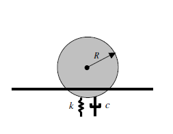
Energy dissipation by friction and inelastic collisions are modeled by spring-dashpot elements. The spring stiffness is a function of the material size and properties such as the Young’s Modulus, and Poisson’s Ratio. Quantifying the energy loss is lumped with the damping effects related to the coefficient of restitution.

Dr. Liz Del Cid

Discrete Element Modeling