Granular Dynamics or Contact Mechanics

October 7, 2018October 7, 2018Leave a comment

I have recently delved deeper into DEM and Powder Mechanics and have spent hours reading conference proceedings and studies. After a while I had to take a step back and answer the basics. Am I studying granular dynamics or contact mechanics?

In truth, both. Granular dynamic is studied as particle kinematics where we obtain the incremental displacements at contact from the contact reactions. During these interactions we look at particle-particle slip, rotation, normal and tangential forces, energy damping forces, chemical and body forces, among other factors which combined reorient the particle and updates it position and displacements.

Contact mechanics is labeled as the theoretical methods used to describe that force-displacement behavior. There are so many theories and I have mentioned a few in previous post. Most restrict the particle considered to spheres and study the force-displacement behavior as dependent on the material properties, size, surface conditions and in some cases the medium in which these material are interacting. Think soil movement vs a fluidized bed.

Needless to say, which model you use will depend on the problem application being studied. I keep on hand about nine different models that are switched out depending on the study being performed. These models also have a number of variation in behavior if I am also observing cohesive/adhesive forces.

Particle size or scale is one of my driving factors when selecting a theory. If the material we are testing and modeling is being handled at the a small sieve size (a few millimeters in diameter) then a model such one by Deresiewicz, Tsuji, or Hertz is used. If we are working at a larger scale, say pellets or bigger, we will look at models by Luding or Walton. It all depends on the material and how it is being handled. Pneumatic conveying, fluidized beds, overland conveying all have their own set of requirements and challenges.

The study of DEM is all about knowing what methods are at your disposal, knowing when and how to use them, and filling in the gaps with further research. I have no one recommended reading, however, Colin Thornton has studied the various methods extensively and recorded his findings. A good place to start is with his Particle Technology Series: Granular Dynamics, Contact Mechanics, and Particle System Simulations–A DEM study.

I am currently reading The Springer Particle Technology Series Volume 24. It may be a little dense if you are just starting your DEM studies but it is a good resource towards other papers that may be better tailored to your application.

Good luck in your studies! Let me know how it is going and reach out on LinkedIn or here.

DEM Particle Characteristic Velocity

November 2, 2017July 31, 2018Leave a comment

The characteristic velocity of a DEM particle is the impact velocity of the particle with a surface and is also known as the drop velocity. The vertical impact velocity is the gravitational potential energy converted to kinetic energy at the instant just pre-impact.

impact velocity

The gravitational potential energy is a function of the particle’s mass and the height from the impact surface as follows:

$U_g = mgh$

Where m, g, and h represent the mass of the particle, the height of impact, and gravity respectively. The kinetic energy just prior to impact is given by the velocity pre-impact as:

$U_k = \frac{1}{2}mV_{impact}^2$

Equating the particle’s initial energy state to the energy state prior to impact will provide the vertical impact velocity (assuming no energy dissipation such as drag)

$\frac{1}{2}mV_{impact}^2 = mgh$

$V_{impact}= \sqrt{2gh}$

Most dynamic textbooks provide collision and projectile problems for practice.

Macroscopic Cohesion

October 11, 2016July 31, 2018Leave a comment

The yield strength of the macro-scale cohesion of particulate materials can be described by Coulomb cohesion. The Mohr-Coulomb failure criterion, described by:

$\sigma_t = \pm (\tan \varphi \ \sigma_n + c)$

divides the mechanical strength of the material into the angle of internal friction and the macroscopic cohesion of the material c [1]. Here $\sigma_n$ and $\sigma_t$ are the normal and tangential stresses. These parameters characterize the material at particular stress states and can extend the effects of cohesion into the elastic domain in the stress plane. The angle of internal friction and the macroscopic cohesion can be determined with physical tests of shear, compression or tension. Particulate materials are typically tested under compressive loading. Under a uniaxial compression test, the yield strength $\sigma_y$ of the material can be derived by:

$\sigma_y = \frac {\cos \varphi}{1- \sin \varphi}c$

The figure provides a graphical representation of Mohr-Coulomb’s criterion where the parameters $\varphi$ and c characterize the strength of the material. The straight line represents the linear failure envelope that is obtained from the shear strength of a material at a particular state of stress in the material.

Morh-Coulomb Criterion [2].

Nedderman R. M., Statics and Kinematics of Granular Materials, Cambridge Univeristy Press, Cambridge, 1992.
Farhang R., Dubois F., Discrete-Element Modeling of Granular Materials, John Wiley & Sons Inc. 2011

Introduction to Cohesive Forces

October 10, 2016July 31, 2018Leave a comment

Cohesive forces stem from cohesive interactions between particles and can typically be classified into three levels of cohesion: adhesion, capillary and cementation [1]. Here, interactions between particles are limited to surface interactions such as in physico-chemical interactions with very short range or through solid or liquid bridges at the particle contact. Electrical forces such as van der Waals forces are considered negligible in macroscale mechanical behavior. This is due to the gravitational forces dominating the bulk forces in material flow. The cohesive forces between contacting particles form an association with the contacting normal force and the contact overlap or separation . Upon the application of a tensile force between the particles, the adhesive force resists the direction of separation and for a distance the bond is still held. The figure below shows two particles in contact through loading and unloading. The cohesive force resists the tensile force. The distance at which the cohesive bond is broken differs from the distance for which the cohesive contact bond is formed. The distance at which the cohesive bond breaks leads to a hysteresis phenomenon.

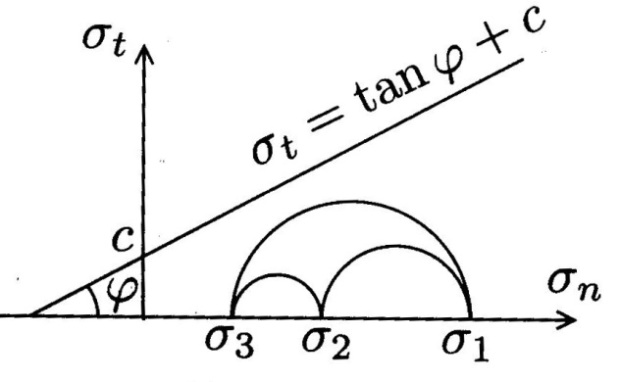
(a) Formation of a cohesive contact. (b) Tensile strength due to the presence of cohesion. (c) Failure of the cohesive bond with a value of $\delta_n$ > 0. (d) The evolution of the normal force as a function $\delta_n$ of $\gamma$ where represents the energy per unit area to break the cohesive contact [1].

[1] Farhang R., Dubois F., Discrete-Element Modeling of Granular Materials, John Wiley & Sons Inc. 2011

The Finnie Model of Erosive Wear

June 9, 2016July 31, 20181 Comment

The following model is what I use for evaluating wear in DEM. It’s based on the work of Iain Finnie.

Finnie I., Erosion of Surfaces by Solid Particles. Wear, 3(2):87-103, 1960.

The wear model I use for granular contact is based on two parts. The first part is the calculation of the number, direction (angle of impact) and velocity of the particles striking the ductile surface. Brittle materials can see fractures upon impact and require a different approach to the mathematical model that is solely based on the material properties and will not be discussed here.

The model assumes ductile material so the model will calculate the amount of surface material removed based on the particle trajectories. Note: the model though it calculates the volume of material removed, the particle velocities are dependent on the material size which is an estimate to begin with so the effect of particle size on erosion is relatively uncertain and is a qualitative approach to wear.

Materials such as steel undergo wear by a process of plastic deformation in which the material is removed by the displacement or cutting action of the eroding particle. The assumptions behind the model are that there is a ratio between the normal force component and the shear component of constant value K. This is true if the particle rotation during the cutting/impact is fairly small. In addition, it is assumed that there is a ratio between the depth of contact $l$ and the depth of cut $y_t$ as seen in the figure below of value $\psi$ .

Wear, 3(1960) 93: Idealized picture of abrasive grain striking a surface and removing material. Initially the velocity of the particle’s center of gravity makes an angle $\alpha$ with the surface.

Further assumptions require that a constant plastic flow stress $p$ is reached immediately upon impact. This is for the traction analysis so that the particle cutting face is of uniform width which is large compared to the depth of cut. The volume of material removed by the particle is then taken as the product of the area swept out by the particle tip and the width of the cutting face.

The cases under which material is removed are as follows:

The particle comes down as a low angle, cuts out part of the surface and then leaves again which means the depth of cut goes to zero as the particle departs.
At the higher angles the horizontal motion of the particle ceases before it leaves the surface so the cutting stops when the velocity goes to zero.

For (1) think of a particle rubbing along the surface when impacting at low angles and the particle striking the surface head on and creating craters for high angle impacts (2).

Integrating over the duration of impact or cutting period provides the following expressions for the volume removed:

$Q = \frac{mV^2}{p \psi K}(\sin 2 \alpha - \frac{6}{K} \sin^2 \alpha)$ if $\tan \alpha \leq \frac{K}{6}$

$Q = \frac{mV^2}{p \psi K}(\frac{K \cos^2 \alpha}{6})$ if $\tan \alpha \geq \frac{K}{6}$

The first equation is for low angle impact, the second for high angle impact. The variables are defined as follows:

$Q$ = the volume of material removed

$m$ = the mass of the particle or effective mass of the particles impacting the surface

$V$ = the velocity of impact

$p$ = constant of plastic flow stress

$\psi$ = ratio of depth of contact to depth of cut

$\alpha$ = angle of impact

$K$ = ratio between the normal force and the shear force

Down side to this model is that the formulation assumes the particle impacts a smooth surface every time when in reality the surface wastes away by previous impacts and becomes rough. Since the surface roughness increases throughout the duration of the impact period there is a correction made to the model. This correction is made under the observation that the surface roughness increases with each impact. Therefore, in an impact with a rough surface more material is removed than from a smooth surface. The second observation is that not all particles that impact the surface will remove material in an idealized manner and can sometimes not remove material at all. Thus by inspection of erosion craters due to a known number of abrasive grain cuts, the volume removed is assumed to be 50% of the predicted erosion.

In addition, $\psi$ , is assumed to be 2 from metal cutting experiments, according to Finnie. This leaves one variable left for the user to define (K). If using K = 2 as approximated from angular abrasive grain erosion tests, the corrected volume removed is approximately defined as follows:

$Q \approx \frac{mV^2}{8p}(\sin 2 \alpha -3 \sin^2 \alpha)$ $\alpha \leq 18.5 ^{\circ}$

$Q \approx \frac{mV^2}{24p} \cos^2 \alpha$ $\alpha \geq 18.5^{\circ}$

Maximum erosion has been observed in the impact angle range of 15-20° so the estimated maximum volume removal is given by

$Q \approx 0.075 (\frac{MV^2}{2}) \frac{I}{p}$

which is 7.5% of the particle’s kinetic energy divided by the flow pressure of the material.

What the I use as an input to the DEM engine is the K variable relating the normal force to the shear force. This is also a measure of the shape of the material impacting the surface. If the material is near spherical the K value will increase, for material that is abrasive (has a rough surface) the K value will be small.

Most abrasive material has a K value in the range of 1.5 to 2.5. Perfectly spherical material would have a K value of 5.0. Studies show that K is approximately 2 for angular abrasive grain. As most material modeled with spherical particles is rough, the K value should be on the lower end of the K value range.

Contact Area of Particle-Plane Impact

June 8, 2016July 31, 20181 Comment

A particle of radius R impacts a wall with some velocity, $V_{impact}$ . The penetration length is defined as $\delta$ . The contact area radius is defined by $a$ .

Using Pythagorean Theore parparimpact m, the contact radius is defined by:

$a^2 + (R - \delta)^2 = R^2$

$a^2 = R^2 - (R-\delta)^2$

$a^2 = R^2 - (R^2 -2R \delta + \delta^2)$

$a^2 = 2R \delta - \delta^2$

If $\delta$ is small then $\delta^2$ is even smaller and we may omit it. Therefore, $a^2 = 2R \delta$ and the cross sectional area is defined by: $A_0 = \pi a^2 = 2 \pi R \delta$ .

Deriving the Damping Coefficient (part 2)

June 8, 2016July 31, 2018Leave a comment

Condition 1: At time = 0 and position y = 0

condition1

$y(0) = e^{- \xi *0} \{Acos( \tilde{ \omega} *0) \ + \ Bsin(\tilde{ \omega} *0 )\}$

$Acos( \tilde{ \omega} *0) \ = \ A(1) \ = \ 0$

Therefore: A = 0

To use the condition of $V_0 \ = \ \dot{y}$ at t = 0, we need to take the first derivative of the position equation

$y(t) = e^{- \xi t} \{Bsin( \tilde{ \omega} t)\}$

$\dot{y}(t) = e^{- \xi t} \frac{d}{dt} \{Bsin( \tilde{ \omega} t)\} + \{Bsin( \tilde{ \omega} t)\} \frac{d}{dt} e^{- \xi t}$

$\dot{y}(t) = e^{- \xi t} \{ \tilde{ \omega} Bcos( \tilde{ \omega} t )\} - \xi \{Bsin( \tilde{ \omega} t) \} e^{- \xi t}$

$\dot{y}(t) = e^{- \xi t} B \{ \tilde{ \omega} cos( \tilde{ \omega} t )- \xi sin( \tilde{ \omega} t) \}$

$V_o = e^{- \xi *0} B \{ \tilde{ \omega} cos( \tilde{ \omega} *0 )- \xi sin( \tilde{ \omega}*0) \}$

$V_0 = B \{ \tilde{\omega}\}$

$B = \frac{V_0}{\tilde{\omega}}$

This brings our position and velocity equations to:

$y(t) = \frac{V_0 e^{- \xi t}}{\tilde{\omega}}sin(\tilde{\omega}t)$

$\dot{y}(t) = \frac{V_0 e^{- \xi t}}{\tilde{\omega}}\{\tilde{\omega} cos( \tilde{\omega}t) - \xi sin(\tilde{\omega}t)\}$

The goal of solving this system is to extract the damping coefficient. To do this, evaluate the system at the instant the particle rebounds from the ground.

condition2

These conditions are: y = 0, $t = t_f$ , $\dot{y} = V_f$

First we need to determine $t = t_f$

condition2b

The equation for position is a sine wave of the form: $y = C \ \ sin(\tilde{\omega}t)$

sinewave

The sine wave has a period T and the time elapsed during that period is T/2, where

period, $T = \frac{2 \pi}{\tilde{\omega}}$

Therefore,

time, $t = \frac{T}{2} = \frac{\pi}{\tilde{\omega}}$

Solving the velocity equation at the determined conditions: $t = \frac{\pi}{\tilde{\omega}}$ , $\dot{y} = V_f$

$y(t) = \frac{V_0 e^{- \xi t}}{\tilde{\omega}}sin(\tilde{\omega}t)$

$V_f = \frac{V_0 e^{- \xi \frac{\pi}{\tilde{\omega}}}}{\tilde{\omega}}\{\tilde{\omega} cos( \tilde{\omega}\frac{\pi}{\tilde{\omega}}) - \xi sin(\tilde{\omega}\frac{\pi}{\tilde{\omega}})\}$

$V_f = \frac{V_0 e^{- \xi \frac{\pi}{\tilde{\omega}}}}{\tilde{\omega}}\{\tilde{\omega} cos( \pi) - \xi sin(\pi)\} = V_0 e^{- \xi \frac{\pi}{\tilde{\omega}}}$

Using this information for $V_f$ and $V_0$ combined with the linear definition of the coefficient of restitution, e, which is given by:

$e = \frac{V_f}{V_o}$

$e = exp^{- \xi \frac{\pi}{\tilde{\omega}}}$

Bringing out system to its initial terms: m, k, c

$ln(e)=- \zeta \omega_0 \frac{\pi}{\omega_0 \sqrt{1 - \zeta^2}}$

$ln(e)=- \zeta \frac{\pi}{\sqrt{1 - \zeta^2}}$

$\sqrt{1 - \zeta^2} ln(e)=- \zeta \pi$

$(\sqrt{1 - \zeta^2}ln(e) )^2= (- \zeta \pi)^2$

$(\sqrt{1-\zeta^2}) [ln(e)]^2 = \pi^2 \zeta^2$

$[ln(e)]^2 - \zeta^2 [ln(e)]^2 = \pi^2 \zeta^2$

$\pi^2 \zeta^2 + \zeta^2 [ln(e)]^2 = [lkn(e)]^2$

$\zeta^2 (\pi^2 + [ln(e)]^2) = [ln(e)]^2$

$\zeta^2 = \frac{[ln(e)]^2}{\pi^2 + [ln(e)]^2}$

Recall:

damping ratio, $\zeta = \frac{c}{C_{crit}} \rightarrow \frac{c}{2 \sqrt{km}}$

$(\frac{c}{2 \sqrt{km}})^2 = \frac{[ln(e)]^2}{\pi^2 + [ln(e)]^2}$

$\sqrt{(\frac{c}{2 \sqrt{km}})^2 }= \sqrt{\frac{[ln(e)]^2}{\pi^2 + [ln(e)]^2}}$

$\frac{c}{2 \sqrt{km}}= \frac{ln(e)}{\sqrt{\pi^2 + [ln(e)]^2}}$

$c = \frac{2\sqrt{km}ln(e)}{\sqrt{\pi^2 + [ln(e)]^2}} = \frac{2\sqrt{km}ln(\frac{1}{e})}{\sqrt{\pi^2 + [ln(\frac{1}{e})]^2}}$

This defines the viscous damping coefficient.

Deriving the Damping Coefficient (part 1)

June 7, 2016July 31, 2018Leave a comment

damp1

$m\ddot{y}\ + c\dot{y}\ + ky\ = 0$ $y\leq 0$

This differential equation can be re-arragned as

$\ddot{y}\ + \frac{c}{m}\dot{y}\ + \frac{k}{m}y\ = 0$ $y\leq 0$

$\ddot{y}\ + \ 2 \zeta \omega_0 \dot{y}\ + \omega_0^2\ y= 0$ $y\leq 0$

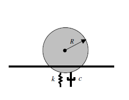
Where $\zeta$ is the relationship between the damping of the system relative to critical damping $\omega_0$ is the natural frequency of simple harmonic oscillation

critical damping coefficient, $C_{crit}\ = 2 \sqrt{km}$

damping ratio, $\zeta = \frac{c}{C_{crit}} \rightarrow \frac{c}{2 \sqrt{km}}$

natural frequency, $\omega_0 = \sqrt{\frac{k}{m}}$

Therefore, $\frac{c}{m}$ can be described by $2 \zeta \omega_0$

$2 \zeta \omega_0 = 2\frac{c}{2 \sqrt{km}} \sqrt{\frac{k}{m}}$

$2 \zeta \omega_0 = \frac{c}{\sqrt{k} \sqrt{m}} \frac{\sqrt{k}}{\sqrt{m}}$

$2 \zeta \omega_0 = \frac{c}{\sqrt{m} \sqrt{m}} \ = \frac{c}{m}$

Solving for the general solution to this system, $\ddot{y}\ + \ 2 \zeta \omega_0 \dot{y}\ + \omega_0^2\ y= 0$ $y\leq 0$

Start by identifying the roots of the system and obtaining the general solution.

Roots of the auxiliary equation

$r^2\ + \ 2 \zeta \omega_0 r \ + \omega_0^2 = 0$

$r = \frac{-2 \zeta \omega_0 \pm \sqrt{(2 \zeta \omega_0)^2 - 4 \omega_0^2}}{2}$

$r = \frac{-2 \zeta \omega_0}{2} \pm \frac{1}{2} \sqrt{4 \zeta ^2 \omega_0^2 - 4 \omega_0^2}$

$r = - \zeta \omega_0 \pm \sqrt{ \zeta ^2 \omega_0^2 - \omega_0^2} \rightarrow \ -\zeta \omega_0 \pm \sqrt{-1} \sqrt{ \omega_0^2 - \zeta ^2 \omega_0^2}$

$r = - \zeta \omega_0 \pm \omega_0 \sqrt{1 - \zeta ^2} i$

General solution to the second order differential equation, $\ddot{y}\ + \ 2 \zeta \omega_0 \dot{y}\ + \omega_0^2\ y= 0$ $y\leq 0$

$y(t) = e^{- \zeta \omega_0 \ t} \{Acos( \omega_0 \sqrt{1 - \zeta ^2} t) \ + \ Bsin( \omega_0 \sqrt{1 - \zeta ^2} t)\}$

Simplify the notation by using $\tilde{ \omega} \ = \omega_0 \sqrt{1 - \zeta ^2}$ and $\xi = \zeta \omega_0$

$y(t) = e^{- \xi t} \{Acos( \tilde{ \omega} t) \ + \ Bsin(\tilde{ \omega} t )\}$

Use the known condition to solve for constant A and B

Defining the Damping Coefficient

June 6, 2016July 31, 2018Leave a comment

damp1

The combined spring-damper contact model can be defined such that the coefficient of the viscous damper c, can be determined in terms of the restitution coefficient e. This is accomplished by solving the differential equation of motion for the particle during the impact and restitution phase. The equation of motion of the particle during the contact is given by

$m\frac{\partial^2 y}{\partial t}\ + c\frac{\partial y}{\partial t}\ + ky\ = 0$

This differential equation can be re-arranged as

$\frac{\partial^2 y}{\partial t}\ +2\xi\frac{\partial y}{\partial t}\ + \omega^2 y\ = 0$

Where $2\xi\ = \frac{c}{m}$ and $\omega^2\ = \frac{k}{m}$ . The mass damping ratio parameter is $\xi$ and $\omega$ is the natural undamped circular frequency of the mass-spring system. The result of this analysis determines the value of viscous damper as a function of particle mass, normal contact stiffness and the coefficient of restitution.

$c\ = \frac{2\sqrt{km}\ln(\frac{1}{e})}{\sqrt{\pi^2\ + (\ln(\frac{1}{e}))^2}}$

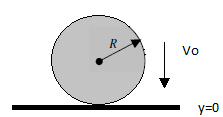
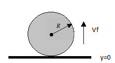
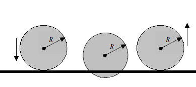
Let the coefficient of restitution e be defined as the absolute value of the normal component of the release velocity $(V_{y}^f)$ to the initial normal component impact velocity $(V_{y}^0)$ . Then the coefficient of restitution e is

$e\ =|\frac{V_{y}^f}{V_{y}^0}|$

A simple check of accuracy when modeling the energy loss during an impact with a coefficient of restitution can be assessed by checking the validity of the equation:

$e\ =\sqrt{\frac{h_{1}}{h_{0}}}$

Where $h_0$ and $h_1$ are the initial height of the ball when released with zero velocity and the maximum height of the ball after impact, respectively.

Choosing a Timestep

April 20, 2016July 31, 2018Leave a comment

DEM algorithms are numerical time integration schemes that perform dynamic updating of the particle’s motion throughout the duration of the simulation. The usual time integration scheme implemented is the explicit central difference procedure and is conditionally stable. This means the time step must provide numerical stability when the contact force is modeled by a linear stiffness. Therefore, the time step needs to be less than 2 over the natural circular frequency of a simple-mass system. It is typically suggested that the step value be about 5-10% of this contact time to prevent erratic behavior in the particle contact. Rule of thumb says there should be at least ten time steps between the initial contact to the rebound of the particle.

Dr. Liz Del Cid

Discrete Element Modeling

Category: DEM Fundamentals