Deriving the Damping Coefficient (part 1)

damp1

m\ddot{y}\ + c\dot{y}\ + ky\ = 0          y\leq 0

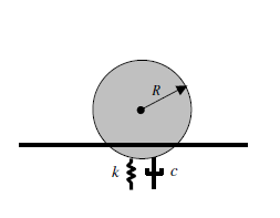
This differential equation can be re-arragned as

\ddot{y}\ + \frac{c}{m}\dot{y}\ + \frac{k}{m}y\ = 0          y\leq 0

or

\ddot{y}\ + \ 2 \zeta \omega_0 \dot{y}\ + \omega_0^2\ y= 0          y\leq 0

Where \zeta is the relationship between the damping of the system relative to critical damping \omega_0 is the natural frequency of simple harmonic oscillation

critical damping coefficient,  C_{crit}\ = 2 \sqrt{km}

damping ratio, \zeta = \frac{c}{C_{crit}} \rightarrow \frac{c}{2 \sqrt{km}}

natural frequency, \omega_0 = \sqrt{\frac{k}{m}}

Therefore, \frac{c}{m} can be described by 2 \zeta \omega_0

2 \zeta \omega_0 = 2\frac{c}{2 \sqrt{km}} \sqrt{\frac{k}{m}}

2 \zeta \omega_0 = \frac{c}{\sqrt{k} \sqrt{m}} \frac{\sqrt{k}}{\sqrt{m}}

2 \zeta \omega_0 = \frac{c}{\sqrt{m} \sqrt{m}} \ = \frac{c}{m}

Solving for the general solution to this system, \ddot{y}\ + \ 2 \zeta \omega_0 \dot{y}\ + \omega_0^2\ y= 0          y\leq 0

Start by identifying the roots of the system and obtaining the general solution.

Roots of the auxiliary equation

r^2\ + \ 2 \zeta \omega_0 r \ + \omega_0^2 = 0

r = \frac{-2 \zeta \omega_0 \pm \sqrt{(2 \zeta \omega_0)^2 - 4 \omega_0^2}}{2}

r = \frac{-2 \zeta \omega_0}{2} \pm \frac{1}{2} \sqrt{4 \zeta ^2 \omega_0^2 - 4 \omega_0^2}

r = - \zeta \omega_0 \pm \sqrt{ \zeta ^2 \omega_0^2 - \omega_0^2} \rightarrow \ -\zeta \omega_0 \pm \sqrt{-1} \sqrt{ \omega_0^2 - \zeta ^2 \omega_0^2}

r = - \zeta \omega_0 \pm \omega_0 \sqrt{1 - \zeta ^2} i

General solution to the second order differential equation, \ddot{y}\ + \ 2 \zeta \omega_0 \dot{y}\ + \omega_0^2\ y= 0          y\leq 0

y(t) = e^{- \zeta \omega_0 \ t} \{Acos( \omega_0 \sqrt{1 - \zeta ^2} t) \ + \ Bsin( \omega_0 \sqrt{1 - \zeta ^2} t)\}

Simplify the notation by using \tilde{ \omega} \ = \omega_0 \sqrt{1 - \zeta ^2} and \xi = \zeta \omega_0

y(t) = e^{- \xi t} \{Acos( \tilde{ \omega} t) \ + \ Bsin(\tilde{ \omega} t )\}

Use the known condition to solve for constant A and B

Defining the Damping Coefficient

damp1

The combined spring-damper contact model can be defined such that the coefficient of the viscous damper c, can be determined in terms of the restitution coefficient e. This is accomplished by solving the differential equation of motion for the particle during the impact and restitution phase. The equation of motion of the particle during the contact is given by

m\frac{\partial^2 y}{\partial t}\ + c\frac{\partial y}{\partial t}\ + ky\ = 0

This differential equation can be re-arranged as

\frac{\partial^2 y}{\partial t}\ +2\xi\frac{\partial y}{\partial t}\ + \omega^2 y\ = 0

Where 2\xi\ = \frac{c}{m} and \omega^2\ = \frac{k}{m}. The mass damping ratio parameter is \xi  and \omega is the natural undamped circular frequency of the mass-spring system. The result of this analysis determines the value of viscous damper as a function of particle mass, normal contact stiffness and the coefficient of restitution.

c\ = \frac{2\sqrt{km}\ln(\frac{1}{e})}{\sqrt{\pi^2\ + (\ln(\frac{1}{e}))^2}}

Let the coefficient of restitution e be defined as the absolute value of the normal component of the release velocity (V_{y}^f) to the initial normal component impact velocity (V_{y}^0). Then the coefficient of restitution e is

e\ =|\frac{V_{y}^f}{V_{y}^0}|

A simple check of accuracy when modeling the energy loss during an impact with a coefficient of restitution can be assessed by checking the validity of the equation:

e\ =\sqrt{\frac{h_{1}}{h_{0}}}

Where  h_0 and h_1 are the initial height of the ball when released with zero velocity and the maximum height of the ball after impact, respectively.