Paul Giroux on civil engineering and construction.
Mr. Giroux, from Kiewit, presented the history and civil engineering marvel of the Hoover Dam. The presentation centered on the excavation and concrete work done by the Six Companies on the Boulder Canyon Project from 1931-1936. Giroux provided an interactive presentation filled with historical pictures of the men working, the machines involved and the engineering plans that brought the project together. The presentation introduced the engineering and construction leaders of the day and laid out their challenges. In addition, it provided a detailed engineering construction approach to the concrete work and technology of the time.
Mr. Giroux began his presentation with a brief history of the U.S. politics of the 1930s. He then introduced the Boulder Canyon Project Act of 1928 which authorized the construction of the Hoover Dam. The massive civil engineering feat was to be constructed in Black Canyon on the Colorado River between Arizona and Nevada. The structure required 3,250,000 cubic yards of concrete and is listed as one of our modern world marvels.
According to Mr. Giroux, the engineering plans were drawn and reviewed by the Bureau of Reclamations. The three major portions and challenges of the project were the diversion of the Colorado River, the construction of the concrete-gravity arch dam and the hydropower plant. Mr. Giroux, in order to provide further knowledge, provided a brief biography of the men in charge of the engineering and construction. He introduced Raymond F. Walter, the Chief Engineer of the Bureau of Reclamations, as the key engineer in the design process and construction bid collection analysis. He also mentioned Frank T. Crowe, the project superintendent, chosen for this work on the nation’s largest dams at that time and John Savage, the engineer in charge of project supervision and onsite design.
The construction bid went to The Six Companies for $48 million which is said came within $25,000 of the estimate made by the Bureau. In order to begin construction, the City of Boulder was developed to house and maintain the community of working men. Once the crews were established, the construction team had 28 months to divert the river by excavating four tunnels. Each tunnel has a 56 foot diameter and together a combined length of approximately three miles. The construction method approach was to drill in the explosives, active them and then haul off the soils and rock. This method required the use of 25 machines and 1,500 men. Once a tunnel was completed, the concrete work began. To provide the necessary material, aggregate, processing and concrete batch plants were developed on low and high ground. Low ground plants were used for the tunnels and base structure. The high ground plants for the rising structure. Several rail lines were also constructed to bring in additives from Las Vegas and the surrounding towns. The concrete pour for each tunnel was divided into 40 foot sections and were composed of the tunnel floor, sidewalls and top arch. To hold the volume of water expected during the flood season, the tunnels were designed be three feet thick. The tunnel concrete lining reduced the tunnel opening to 50 feet.
Once the tunnels were completed, river diversion and construction of the upstream and downstream cofferdams began. To meet the project milestones, work had to continue 24 hours a day in three consecutive shifts. The size of each cofferdam was twice the base structure size of the Hoover Dam, a conservative was measurement made to prevent flooding of the construction site and injury to the men. Once the pumping of water was completed the form work of the base structure was started. The concrete gravity arch dam was to be built in sections. To tackle the problem of concrete shrinkage, a method for removing the heat produced by the concrete needed to be developed. Engineer John Savage proposed the winning design in which one inch pipe was weaved into the sections and concrete pour around it. To lower the thermal stress and expedite concrete shrinkage, river water and then ice water was pumped throughout each section. As the shrinkage settled, grout was pumped under pressure and the pipes filled. Two 20 ton cableway cranes were used for the placement of concrete in the actual dam. Mr. Giroux said the civil engineering marvel of the Hoover Dam does not stop at the massive tunnel excavation and concrete pour. The construction of the hydropower plant proved to take longer than the construction of the dam itself. The power house holds 17 turbines, all of which had to be assembled on site.
In concluding his presentation, Mr. Giroux gave a brief history of the labor laws of the time and commemorated the lives lost in the pursuit of restraining the Colorado River. He then proceeded to answer questions regarding the curing process of the dam, which he said is still curing. Comparisons were then made between dirt dams, concrete gravity arch dams and buttress dams.
For further reading consider the following:
- Dolen, T.P, P.E., “Advances in Mass Concrete Technology-The Hoover Dam Studies”, Concrete Technology, ASCE, Pages 58-73, 2010.
- Rogers, J.D., P.E, “Hoover Dam: Evolution of the Dam’s Design”, Structural Engineering and Hydraulics, ASCE, Pages 85-123. 2010.
- Bartojay, K P.E., Joy, Westin, “Long-Term Properties of Hoover Dam Mass Concrete”, Concrete Technology, ASCE. Pages 74-84. 2010.
 and the depth of cut
  as seen in the figure below of value
  .
.
 with the surface.
 is reached immediately upon impact. This is for the traction analysis so that the particle cutting face is of uniform width which is large compared to the depth of cut. The volume of material removed by the particle is then taken as the product of the area swept out by the particle tip and the width of the cutting face.
 if
if 
 if
if 
 = the volume of material removed
 = the mass of the particle or effective mass of the particles impacting the surface
 = the velocity of impact
 = constant of plastic flow stress
 = ratio of depth of contact to depth of cut
 = angle of impact
 = ratio between the normal force and the shear force


 . The penetration length is defined as
  . The contact area radius is defined by
  .
. m, the contact radius is defined by:


 is even smaller and we may omit it. Therefore,
  and the cross sectional area is defined by:
  .
.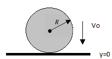


 at t = 0, we need to take the first derivative of the position equation


 ,
, 


 ,
, 

 and
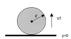
and  combined with the linear definition of the coefficient of restitution, e, which is given by:


![(\sqrt{1-\zeta^2}) [ln(e)]^2 = \pi^2 \zeta^2](https://s0.wp.com/latex.php?latex=%28%5Csqrt%7B1-%5Czeta%5E2%7D%29+%5Bln%28e%29%5D%5E2+%3D+%5Cpi%5E2+%5Czeta%5E2&bg=f3f3f3&fg=404040&s=0&c=20201002)
![[ln(e)]^2 - \zeta^2 [ln(e)]^2 = \pi^2 \zeta^2](https://s0.wp.com/latex.php?latex=%5Bln%28e%29%5D%5E2+-+%5Czeta%5E2+%5Bln%28e%29%5D%5E2+%3D+%5Cpi%5E2+%5Czeta%5E2&bg=f3f3f3&fg=404040&s=0&c=20201002)
![\pi^2 \zeta^2 + \zeta^2 [ln(e)]^2 = [lkn(e)]^2](https://s0.wp.com/latex.php?latex=%5Cpi%5E2+%5Czeta%5E2+%2B+%5Czeta%5E2+%5Bln%28e%29%5D%5E2+%3D+%5Blkn%28e%29%5D%5E2&bg=f3f3f3&fg=404040&s=0&c=20201002)
![\zeta^2 (\pi^2 + [ln(e)]^2) = [ln(e)]^2](https://s0.wp.com/latex.php?latex=%5Czeta%5E2+%28%5Cpi%5E2+%2B+%5Bln%28e%29%5D%5E2%29+%3D+%5Bln%28e%29%5D%5E2&bg=f3f3f3&fg=404040&s=0&c=20201002)
![\zeta^2 = \frac{[ln(e)]^2}{\pi^2 + [ln(e)]^2}](https://s0.wp.com/latex.php?latex=%5Czeta%5E2+%3D+%5Cfrac%7B%5Bln%28e%29%5D%5E2%7D%7B%5Cpi%5E2+%2B+%5Bln%28e%29%5D%5E2%7D&bg=f3f3f3&fg=404040&s=0&c=20201002)

![(\frac{c}{2 \sqrt{km}})^2 = \frac{[ln(e)]^2}{\pi^2 + [ln(e)]^2}](https://s0.wp.com/latex.php?latex=%28%5Cfrac%7Bc%7D%7B2+%5Csqrt%7Bkm%7D%7D%29%5E2+%3D%C2%A0%5Cfrac%7B%5Bln%28e%29%5D%5E2%7D%7B%5Cpi%5E2+%2B+%5Bln%28e%29%5D%5E2%7D&bg=f3f3f3&fg=404040&s=0&c=20201002)
![\sqrt{(\frac{c}{2 \sqrt{km}})^2 }= \sqrt{\frac{[ln(e)]^2}{\pi^2 + [ln(e)]^2}}](https://s0.wp.com/latex.php?latex=%5Csqrt%7B%28%5Cfrac%7Bc%7D%7B2+%5Csqrt%7Bkm%7D%7D%29%5E2+%7D%3D+%5Csqrt%7B%5Cfrac%7B%5Bln%28e%29%5D%5E2%7D%7B%5Cpi%5E2+%2B+%5Bln%28e%29%5D%5E2%7D%7D&bg=f3f3f3&fg=404040&s=0&c=20201002)
![\frac{c}{2 \sqrt{km}}= \frac{ln(e)}{\sqrt{\pi^2 + [ln(e)]^2}}](https://s0.wp.com/latex.php?latex=%5Cfrac%7Bc%7D%7B2+%5Csqrt%7Bkm%7D%7D%3D+%5Cfrac%7Bln%28e%29%7D%7B%5Csqrt%7B%5Cpi%5E2+%2B+%5Bln%28e%29%5D%5E2%7D%7D&bg=f3f3f3&fg=404040&s=0&c=20201002)
![c = \frac{2\sqrt{km}ln(e)}{\sqrt{\pi^2 + [ln(e)]^2}} = \frac{2\sqrt{km}ln(\frac{1}{e})}{\sqrt{\pi^2 + [ln(\frac{1}{e})]^2}}](https://s0.wp.com/latex.php?latex=c+%3D%C2%A0%5Cfrac%7B2%5Csqrt%7Bkm%7Dln%28e%29%7D%7B%5Csqrt%7B%5Cpi%5E2+%2B+%5Bln%28e%29%5D%5E2%7D%7D+%3D+%5Cfrac%7B2%5Csqrt%7Bkm%7Dln%28%5Cfrac%7B1%7D%7Be%7D%29%7D%7B%5Csqrt%7B%5Cpi%5E2+%2B+%5Bln%28%5Cfrac%7B1%7D%7Be%7D%29%5D%5E2%7D%7D&bg=f3f3f3&fg=404040&s=0&c=20201002)
